Optimal Charge Security Camera
Contributors
Abstract
Carbon awareness is becoming increasingly important in the modern world, and many companies are striving to be carbon-neutral in their operations. Existing research into carbon-aware computing has focused on high-power, high-performance computing systems, but there has not been any awareness into carbon-aware battery charging, especially for small-scale IoT devices. In this paper, we propose a controller framework for a battery-powered security camera that balances the tradeoff betweenaccuracy, latency, carbon footprint, and charging decisions based on a pre-defined reward function. This controller picks the optimal models and when to charge every task interval over a horizon of time.
1. Introduction
1.1 Motivation & Objective
While significant research has addressed carbon-aware computing in data centers and high-performance systems, small-scale IoT devices remain overlooked. Battery-powered devices with flexible charging represent a massive, untapped opportunity for carbon optimization. If they are plugged in all the time, they can charge even when it is not carbon-efficient to do so.
Our objective is to develop an intelligent controller that optimizes both computational (which model to select) and charging decisions for battery-powered security cameras. With this approach, we can charge when it is more carbon-efficient, rather than always charging regardless of the carbon cost. We balance our model selection to account for this carbon-efficiency
Because there are differences of opinion on how much each factor (accuracy, latency, carbon footprint, camera uptime) matters to an individual, we define a specific reward function that balances these factors. The system supports dynamic weights, so if the initial weights are not balanced to a specifc use-case, they are adjustable for other use-cases.
For a full breakdown of how we restricted the optimization to solve this problem easier, see Section 3.2.
1.2 State of the Art & Its Limitations
Current carbon-aware research is focused around data-center energy considerations. Data centers incur large electricity costs and carbon emissions. There are 2 main works related to this:
- Carbon- and Precedence-Aware Scheduling for Data Processing Clusters[2] - This paper is focused on scheduling data center workloads such that time requirements are met, but we delay lower priority tasks to carbon-efficient times.
- Carbon-Aware Workload Management in Data Centers[3] - This paper is focused on integrating energy components besides the grid, such as cooling, heating, solar panels, batteries, energy storage, heat pumps, and heating connections to maintain existing data-center workloads while minimizing carbon emissions.
Both of these papers focus on large scale systems with large scale workloads. These approachs are not directly applicable to small-scale IoT devices, which have very limited bandwitdh and very small battery capacity (energy storage).
1.3 Novelty & Rationale
Our approach relies on imitating an Oracle controller. This Oracle controller can see into the future and has full knowledge of the carbon timeseries before it occurs. Using that knowledge, we can solve the full discrete MDP based on the system state over a given finite horizon of time. We can then train a neural network to imitate this Oracle Controller, giving us a controller that can make decisions in real-time.
Additionally, as carbon energy generally follows a sinusoidal pattern, we can leverage this neural network to also gain insight on the ebb and flow of carbon timeseries, further giving us more optimization potential.
Finally, by modelling this problem as an MDP (and POMDP), we can take advantage of existing solving techniques (ex. Data-driven Planning via Imitation Learning[4]), which are well-studied and have multiple proven solutions.
1.4 Potential Impact
This system could easily be extended to other battery-powered devices that make decisions. Any system with a form of energy storage and energy input can take advantage of our models to create their own controllers that balance clean energy.
1.5 Challenges
Implementing an energy-aware decision-making controller for battery-powered edge devices presents several challenges. The primary difficulty is solving and generating sufficient training data from the Oracle MDP, as the state and action spaces grow quickly even under coarse discretization. Specific examples include:
- Deciding how static or dynamic the system should be to user-input. We can allow the user to dynamically adjust their requirements during runtime, but adjusting an already trained controller could be time-consuming, complex, or expensive, especially as we still have to maintain our task interval.
- Discretization of continuous variables. More precision means more runtime, but too much precision can make simple calculations more complex due to floating point errors.
- Carbon patterns vary from region to region. As such, we need to ensure as vast of variety carbon data as possible from different times of the year for a complete picture.
1.6 Metrics of Success
We compare our trained Imitation (Custom) Controller to the Oracle controller over the following metrics:
- Accuracy - how many times over the horizon does the model selected meet the user's requirements?
- Success - number of times the selected model met the user's requirements, and had enough energy to run.
- Small Miss - number of times the selected model didn't meet the user's requirements, and had enough energy to run.
- Failure - number of times a model was unable to run, due to a lack of energy.
- Utility - differences in the rewards of the Oracle Controller (Section 3.3), the Imitation (Custom) Controller (Section 3.4), and Naive Controller (Section 3.5) decisions over each horizon.
- "Feasibility-Normalized Effective Uptime" - at each timestep \( t \), let \( F_t \) be the set of models feasible under the current energy constraint, and let \( a_t^* = \max_{m \in F_t} a(m) \) be the best achievable accuracy. If a model \( m_t \) is selected and runs, the timestep is scored as \( \frac{a(m_t)}{a_t^*} \); if no model is ran (Failure) it scores a \( 0 \). The metric is computed as the average score over the horizon.
3. Technical Approach
3.1 Model Profiler
To simplify the optimization, we benchmarked and created model profiles separately before our simulation loop. The main simulation loop then uses these pre-computed profiles to make decisions at runtime. We do NOT separately profile during the simulation itself, which is a known limitation. See Section 5.3 for more information.YOLOv10 Power and Latency Measurement
A Model task is defined as loading an image and running the default classifier function on it. The task involves:
model-profiler/power_profiler.py:277
start_time ← current_time()

FOR i ← 1 TO iterations DO
    avg_power ← measure_with_powermetrics(inference_task)
    append avg_power to inference_powers
    sleep for 4 seconds
END FOR

end_time ← current_time()
total_duration ← end_time - start_time

total_delay_time ← iterations x 4.0
actual_inference_duration ← total_duration - total_delay_time
avg_inference_time_seconds ← actual_inference_duration / iterations
During this task, the power profiler measures:
- Power consumption: Baseline, idle, and inference power in milliwatts using macOS powermetrics
- Energy efficiency: Energy per inference in mWh calculated from power draw and inference time
- Performance metrics: Inference time, success rate, detection count
- Model variants: All YOLOv10 versions (N, S, M, B, L, X)
The profiler uses powermetrics with sudo access to capture CPU/GPU/ANE
power consumption during the model task, storing results in
model-profiler/power_profiles.json. Each model is benchmarked across 1000 iterations with outlier removal for stable
baseline measurements. Time per inference is tracked to store latency information
alongside power data. Outlier removal trims the top and bottom 20% of power readings
to eliminate anomalies and uses median values for robust statistics.
YOLOv10 Accuracy
Model accuracy values are extracted from the COCO dataset benchmark results stored in model-data.csv. The dataset contains COCO mAP 50-95 scores for each YOLOv10 model variant, provided by Ultralytics official documentation.
The accuracy analysis processes the CSV data to provide approximate accuracy values for each YOLOv10 model version, enabling the controller to make informed tradeoffs between detection accuracy and energy consumption. We normalize these values by performing \( \text{NormalizedAccuracy} = \frac{\text{COCOmAP5095}}{57.0} \) to get a value between \([0, 1]\) for all models.
3.2 System Parameters (per Controller)
Let the system parameters be:
\[ \Theta = (B_{\max}, r_{\text{chg}}, \Delta, T, \{d_t\}_{t=0}^{T-1}, u_{\text{acc}}, u_{\text{lat}}, \mathcal{M}, E(m), W, X, Y, Z) \]
Where:
- \(B_{\max}\) (mWh): maximum battery capacity
- \(\Delta\) (seconds): task interval (e.g. 300s)
- \(T\) (seconds): horizon length (e.g. 86400s)
- \(d_t \in [0,1]\): dirty energy fraction at timestep \(t\)
-
\(\mathcal{M}\): model profile set, where each profile is \((m_{\text{acc}},
m_{\text{lat}})\) with:
- \(m_{\text{acc}} \in [0,1]\): model accuracy, where \(\text{MAX\_ACC} = \max_{m \in \mathcal{M}} m_{\text{acc}}\)
- \(m_{\text{lat}}\) (seconds): model latency, where \(\text{MIN\_LAT} = \min_{m \in \mathcal{M}} m_{\text{lat}}\)
- \(E(m)\): energy function that maps model \(m\) to its energy consumption in mWh, where \(\text{ENERGY\_MIN} = \min_{m \in \mathcal{M}} E(m)\)
- \(u = (u_{\text{acc}}, u_{\text{lat}}) \in U = \{(u_{\text{acc}}, u_{\text{lat}}) \in \mathbb{R}^2 \mid u_{\text{acc}} < \text{MAX\_ACC}, u_{\text{lat}} > \text{MIN\_LAT}\}\): user requirements, where \(u_{\text{acc}} \in [0,1]\) is the accuracy requirement, and \(u_{\text{lat}}\) (seconds) is the latency requirement
- \(r_{\text{chg}}\) (mWh/s): battery energy added per second
-
\(W, X, Y, Z > 0\): reward function weights representing user preferences:
- \(W\): weight for running a model that successfully meets requirements
- \(X\): penalty weight for "small misses" (selected model successfully executed, but it did not meet the accuracy or latency requirements)
- \(Y\): penalty weight for "large misses" (no model was selected due to insufficient battery capacity)
- \(Z\): penalty weight for amount of dirty energy consumed
3.3 Oracle Controller
The oracle controller has full knowledge of the future carbon trajectory \(\{d_t\}_{t=0}^{T-1}\) over the planning horizon.
State Space
\[ {s} = (t, B_t) \in \mathcal{S} = \{(t, B_t) \mid t \in \{0,\ldots,T-1\},\; B_t \in [0, B_{\max}]\} \]
Where \(t\) denotes the current timestep index and \(B_t\) (mWh) denotes the current battery level.
This state representation is minimal: it includes exactly the variables that affect future feasibility and decision-making. In particular, the oracle's knowledge of the carbon trajectory is encoded implicitly through the timestep index \(t\), as the dirty energy fraction \(d_t\) is a known exogenous function of time.
Action Space
\[ a_t = (m_t, c_t) \in \mathcal{A} = (\mathcal{M} \cup \{\varnothing\}) \times \{0,1\} \]
Each action is \(a_t = (m_t, c_t)\), where \(m_t\) is the model selected for execution (or \(\varnothing\) if no model is executed), and \(c_t\) indicates whether the system charges during the current task interval.
Transition Probability
Given state \(s_t = (t, B_t)\) and action \(a_t = (m_t, c_t)\), the transition probability to successor state \(s_{t+1} = (t', B')\) is defined as:
\[ P(s_{t+1} \mid s_t, a_t) = \begin{cases} 1 & \text{if } t' = t + 1, B_t + c_t \cdot r_{\text{chg}} \ge E(m_t), B' = \min\!\left(B_{\max},\, B_t + c_t \cdot r_{\text{chg}} - E(m_t)\right)\\[6pt] 0 & \text{otherwise.} \end{cases} \]
Thus, all feasible actions induce a deterministic transition with probability one, while actions that would result in negative battery energy are assigned zero probability and are therefore infeasible.
Reward Function
At each timestep, the environment produces outcome indicators based on the chosen action:
- \( \text{success}_t = \mathbf{1}\{m_t \neq \varnothing \wedge \text{acc}(m_t) \ge u_{\text{acc}} \wedge \text{lat}(m_t) \le u_{\text{lat}}\} \)
- \( \text{small\_miss}_t = \mathbf{1}\{m_t \neq \varnothing \wedge (\text{acc}(m_t) < u_{\text{acc}} \vee \text{lat}(m_t) > u_{\text{lat}})\} \)
- \( \text{large\_miss}_t = \mathbf{1}\{m_t = \varnothing\} \)
The dirty energy incurred at timestep \(t\) is:
\[ \Delta D_t = c_t \cdot r_{\text{chg}}\cdot \Delta \cdot d_t. \]
Where \(c_t\) is the charge decision (0 or 1), \(r_{\text{chg}}\) is the charging rate, \(\Delta\) is the task interval, and \(d_t\) is the percent of energy that is dirty at that time.
The immediate reward is defined as:
\[ R(s_t,a_t,s_{t+1}) = W \cdot \text{success}_t - X \cdot \text{small\_miss}_t - Y \cdot \text{large\_miss}_t - Z \cdot \Delta D_t. \]
The optimization objective is to maximize the cumulative reward over the planning horizon. As a result, the total contribution of successes, misses, and carbon cost depends only on their aggregate counts and total dirty energy consumed, not on the specific timesteps at which they occur. In particular, for fixed carbon intensity, a success followed by a miss yields the same cumulative reward as a miss followed by a success, and the timing of a success within the horizon does not affect its contribution as long as feasibility is maintained.
Cumulative quantities such as total successes, misses, or dirty energy consumed are not included in the state. These quantities are only used to compute the cumulative sum of per-step rewards and do not influence future system dynamics or feasibility. Because carbon cost is modeled as a soft penalty and does not constrain future actions, histories that reach the same state \((t,B_t)\) differ only by an additive constant in accumulated reward. Consequently, the optimal continuation from a given state depends solely on the remaining horizon and current battery level, preserving the Markov property without explicitly storing historical metrics in the state.
Objective
The oracle policy \(\pi^*\) maximizes the cumulative reward over the horizon:
\[ \pi^* = \arg\max_{\pi} \sum_{t=0}^{T-1} R(s_t, \pi(s_t), s_{t+1}). \]
This optimization is solved exactly using finite-horizon dynamic programming.
-
Policy Lookup with K-Nearest Neighbors:
- The simulation uses battery discretization with \(F \in \mathbb{R}\) mWh steps for computational efficiency in dynamic programming, while maintaining continuous battery values in state transitions.
- The simulation uses a K-nearest neighbor approach with parameter \(K \in \mathbb{N}_{odd}, K > 0\) to find the nearest discretized battery level with feasible actions. The algorithm identifies the K closest battery levels and selects the first one that has valid feasible actions. If fewer than K feasible options are found within the initial search radius, the algorithm expands the search radius incrementally until exactly K valid options are identified. This ensures robust policy extraction while maintaining optimality within the expanded search space.
-
End Look-ahead for Complete Policy Coverage:
- To ensure optimal policies exist for all reachable states at the final timestep, the oracle computes one extra timestep beyond the planning horizon. This enhancement guarantees complete policy coverage while maintaining correct terminal conditions.
// Enhanced DP with Extra Timestep for Complete Policy Coverage
FOR t ← T DOWNTO 0 DO  // Include extra timestep T for complete coverage
    FOR each battery_level b IN reachable_states DO
        best_value ← -∞
        best_action ← null

        FOR each action a IN feasible_actions(b) DO
            next_state ← transition(t, b, a)
            reward ← R(t, b, a, next_state)

            // Use extra timestep values for complete lookahead
            IF t < T THEN
                future_value ← V[t+1][knn(battery_key(next_state))]
            ELSE
                future_value ← 0  // True terminal value
            END IF

            total_value ← reward + future_value

            IF total_value > best_value THEN
                best_value ← total_value
                best_action ← a
            END IF
        END FOR

        V[t][battery_key(b)] ← best_value
        π[t][battery_key(b)] ← best_action
    END FOR
END FOR
The oracle controller implementation can be found in oracle.py.
3.4 Custom Controller (POMDP, Imitation Learning)
The custom controller operates without access to the future carbon trajectory \(\{d_t\}_{t=0}^{T-1}\) available to the oracle (Section 3.3). At each timestep, it must make decisions based only on real-time observations. As a result, the control problem is naturally modeled as a Partially Observable Markov Decision Process (POMDP).
State Space, Action Space, Transition Probability, and Reward Function
The state space \(\mathcal{S}\), action space \(\mathcal{A} = (\mathcal{M} \cup \{\varnothing\}) \times \{0,1\}\), transition probability \(P(s_{t+1} \mid s_t, a_t)\), and reward function \(R(s_t, a_t, s_{t+1})\) are defined exactly as in Section 3.3. The custom controller operates in the same underlying MDP; only its observability differs.
Observation Space
At each timestep \(t\), the controller receives the observation:
\[ o_t = (B_t, d_t, \Delta d_t) \in \mathcal{O} = [0, B_{\max}] \times [0,1] \times [-1,1], \]
where \(B_t\) is the current battery level, \(d_t\) is the instantaneous dirty energy fraction, and \(\Delta d_t = d_t - d_{t-1}\) captures the change in carbon intensity since the previous timestep. The controller does not observe the timestep index \(t\) or any future carbon values \(\{d_{t'}\}_{t' > t}\).
The inclusion of \(\Delta d_t\) provides a minimal trend signal, allowing the controller to infer short-term carbon dynamics using only locally available information. Unlike the oracle, which implicitly accesses the full trajectory through \(t\), the custom controller must reason about carbon evolution from this limited window.
Policy Learning via Imitation
Rather than attempting to solve the POMDP via belief-state planning, we learn the custom controller via imitation learning using the oracle policy \(\pi^*\) (Section 3.3) as an expert.
To simplify this problem, we assume that ALL system parameters in Section 3.2 are constant per controller (EXCEPT \(\{d_t\}_{t=0}^{T-1}\)). If any of these parameters change, the controller will need to be solved and retrained again. See Section 5.3 for more information.Training Data Generation
To create training data for the custom controller, the oracle solver's optimal decisions must be translated into observation-action pairs that the imitation learning algorithm can learn from. This process extracts the oracle's state-action trajectories and converts them into the observation space that the custom controller will actually encounter at runtime.
The training data generation process works as follows:
FOR each optimal trajectory τ FROM oracle solver DO
    observations ← []
    actions ← []

    FOR each timestep t IN τ DO
        state, action ← τ[t]

        // Extract carbon information
        carbon_intensity ← carbon_data[t]  // [0,1]
        carbon_change ← carbon_data[t] - carbon_data[t-1]  // [-1,1]

        // Normalize battery level for observation space
        normalized_battery ← state.battery_level / B_max  // [0,1]

        // Create observation vector (3D)
        observation ← [normalized_battery, carbon_intensity, carbon_change]

        // Encode action as discrete targets
        model_index ← index_of(action.model)  // 0-6 for YOLOv10 variants
        charge_decision ← int(action.charge)  // 0 or 1

        // Append to training dataset
        observations.append(observation)
        actions.append([model_index, charge_decision])
    END FOR

    // Save as compressed numpy arrays with metadata
    save_training_chunk(observations, actions, trajectory_metadata)
END FOR
Implementation: data/oracle_runner.py:70 and simulation/controllers/oracle.py:504
- Observation Space Translation: The oracle has full knowledge of the timestep \(t\) and future carbon trajectory, but the custom controller only observes \((B_t, d_t, \Delta d_t)\). The training data generation extracts exactly what the custom controller will see at runtime.
- Action Encoding: Model selection is encoded as discrete indices (0-6) corresponding to YOLOv10 variants, while charging decisions become binary targets (0/1).
- Normalization: Battery levels are normalized to \([0,1]\) to make the neural network training stable across different battery configurations.
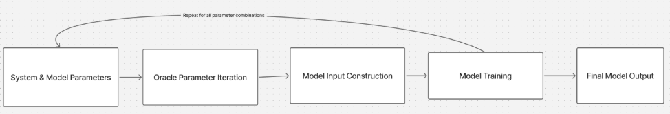
Training Pipeline: Data generation, neural network training, and model evaluation process.
Neural Network Architecture Design
The custom controller uses a 3-layer feedforward network processing 3-dimensional observations: battery level, carbon intensity, and carbon change. The network outputs 8 dimensions: 7 model logits + 1 charge logit.
PolicyNetwork Architecture:
Input Layer: 3 features
Hidden Layer 1: 64 neurons, ReLU activation
Hidden Layer 2: 32 neurons, ReLU activation
Output Layer: 8 neurons (7 model + 1 charge)

Forward Pass:
shared_output = Sequential(Input → Linear(3,64) → ReLU → Linear(64,32) → ReLU → Linear(32,8))
model_logits = shared_output[:, :7]
charge_logit = shared_output[:, 7:]
Implementation: training/train.py
Model selection uses cross-entropy loss, charging decision uses binary cross-entropy loss. Final loss combines both with equal weighting.
The architecture consists of multiple hidden layers with ReLU activations, culminating in a dual-head output structure. One head produces logits for discrete model selection across available YOLOv10 variants, while the other head generates a continuous signal for the charging decision. This design enables the network to learn separate representations for model selection and energy management strategies.
We incorporate feasibility-aware inference design to ensure safety in critical applications. The network predictions are validated against system constraints before execution, with mechanisms to handle prediction failures gracefully.
Per-Controller Training Approach
Each system configuration receives its own neural network rather than one generalized model. This approach was selected to save time with training data generation. See Section 5.3 for more information.
Training Algorithm:
FOR each controller configuration DO
    Initialize fresh PolicyNetwork
    Set optimizer = Adam(lr=0.001)
    Set criterion = CombinedLoss(0.5 * CE_model + 0.5 * BCE_charge)

    FOR epoch = 1 TO 100 DO
        Train on batches of size 32
        Evaluate on validation set
        IF val_loss doesn't improve for 10 epochs THEN
            Break (early stopping)
        END IF
    END FOR
    Save best checkpoint
END FOR
Implementation: training/train.py
Loss combines model selection cross-entropy and charging binary cross-entropy with equal (0.5 each) weighting. Early stopping uses patience of 10 epochs with minimum delta of 0.001.
Integration with Simulation Framework
Inference Pipeline:
Load trained model checkpoint
Set model to eval mode
FOR each timestep DO
    obs = preprocess([battery_level, carbon_intensity, carbon_change])
    model_logits, charge_logit = model(obs)

    model_pred = argmax(model_logits)
    charge_pred = sigmoid(charge_logit) > 0.5

    IF prediction_infeasible THEN
        (NO_MODEL, 0) selected
    END IF
END FOR
Implementation: simulation/controllers/ml_controller.py
Preprocessing normalizes battery level to [0,1] and calculates carbon change. Postprocessing converts model prediction to YOLOv10 variant and applies threshold to charge decision. If there is not enough battery to perform the selected action, the policy falls back to \((\text{NO\_MODEL}, 0)\).
3.5 Naive Controller
We implement a naive baseline controller with a fixed, myopic policy that ignores carbon intensity and does not optimize over the horizon. The controller operates under the same system dynamics as defined in Section 3.2.
Policy
At each timestep \(t\), the naive controller selects an action \(a_t = (m_t, c_t)\) as follows:
- Select the lowest-energy model in \(\mathcal{M}\) that satisfies \((u_{\text{acc}}, u_{\text{lat}})\). If sufficient battery energy is available, execute the model without charging.
- If insufficient battery energy is available to run that model, select the lowest-energy model in \(\mathcal{M}\) regardless of requirements and charge during the interval.
- If insufficient battery energy is available to execute any model, select no model and charge during the interval.
The naive controller code can be found in naive.py.
3.6 Simulation Setup
Configuration Management
Each custom controller is trained on a specific set of system parameters and cannot operate outside those constraints. The simumlation loads the custom controller corresponding to the system parameters to ensure fair comparison across all controllers. See Section 5.3 for more information.
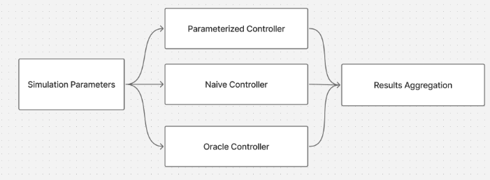
Simulation Pipeline: Controller comparison framework and result aggregation workflow.
Main Simulation Loop
For each unseen test day, the simulation runs all three controllers simultaneously using the same carbon intensity trace and initial conditions. Each controller makes decisions at every task interval based on its available information: the oracle has full future carbon knowledge, the naive controller uses only current battery state, and the custom controller uses real-time observations.
FOR timestep FROM 0 TO horizon_length-1 DO
    current_state ← (timestep, battery_level)

    FOR each controller IN controllers DO
        action ← controller.select_action(current_state)

        IF action.is_feasible(current_state) THEN
            next_state ← transition(current_state, action)
            reward ← calculate_reward(action, next_state)
            path[controller].add(current_state, action, reward)
        ELSE
            handle_infeasible_action(controller, current_state)
        END IF
    END FOR

    update_all_battery_states()
END FOR
Result Aggregation
After completing the simulation horizon, results are aggregated for each controller. Performance metrics include total cumulative reward, success rates, charging patterns, and model usage statistics. The comparison evaluates how well the custom controller approximates oracle performance while respecting real-time constraints.
FOR each controller IN controllers DO
    total_reward ← sum(path[controller].rewards)
    success_rate ← count(path[controller].actions WHERE meets_requirements) / total_actions
    utility_metrics ← calculate_utility(path[controller])

    record_performance(controller, total_reward, success_rate, utility_metrics)
END FOR

generate_comparative_analysis(controllers)
Implementation: simulation/run.py
4. Evaluation & Results
4.1 Results Parameters
Below are all the parameter settings used to generate the results.
Model Profiler Configuration
model-profiler/model.config.json
Model Profiling ParametersPower measurement configuration for model profiling.
{
  "iterations": 1,
  "iter_sleep_sec": 4.0
}
YOLOv10 Model Specifications
model-profiler/power_profiles.json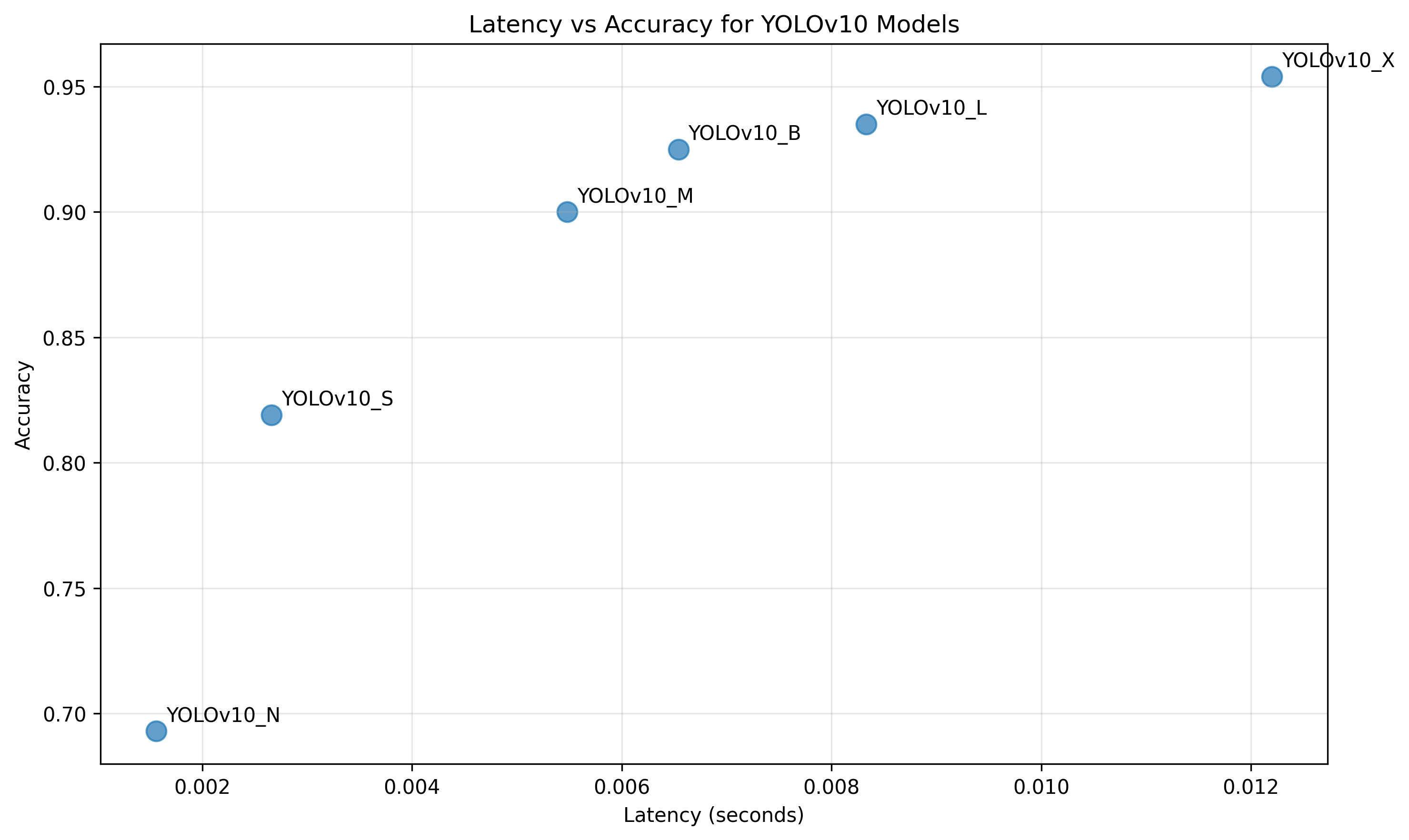
| Model | Energy per Inference (mWh) | Latency (s) | Normalized Accuracy [0,1] |
|---|---|---|---|
| YOLOv10_N | 1.02 | 0.00156 | 0.693 |
| YOLOv10_S | 1.99 | 0.00266 | 0.819 |
| YOLOv10_M | 2.95 | 0.00548 | 0.900 |
| YOLOv10_B | 3.89 | 0.00654 | 0.925 |
| YOLOv10_L | 4.69 | 0.00833 | 0.935 |
| YOLOv10_X | 6.06 | 0.0122 | 0.954 |
Data Configuration
System Constants\(\Delta\), \(T\), \(F\), \(K\)
{
  "task_interval_seconds": 3600, // 1 hour
  "horizon_seconds": 86400,      // 24 hours
  "battery_discretization_step": 0.01,
  "nearest_neighbor_k": 3
}\(u_{\text{acc}}\), \(u_{\text{lat}}\)
[
  {
    "accuracy_threshold": 0.95,
    "latency_threshold_seconds": 0.015
  },
  {
    "accuracy_threshold": 0.819,
    "latency_threshold_seconds": 0.006
  }
]\(W\), \(X\), \(Y\), \(Z\)
[
  {
    "success_weight": 20,
    "small_miss_weight": 5,
    "large_miss_weight": 8,
    "carbon_weight": 7
  },
  {
    "success_weight": 5,
    "small_miss_weight": 7,
    "large_miss_weight": 10,
    "carbon_weight": 15
  }
]\(B_{\max}\), \(r_{\text{chg}}\)
[
  {
    "battery_capacity_mwh": 610,           // 10 YOLOv10_X iterations
    "charge_rate_mwh_per_second": 0.000269 // 3600s -> 95% capacity to run YOLOv10_N
  },
  {
    "battery_capacity_mwh": 105,           // 10 YOLOv10_N iterations
    "charge_rate_mwh_per_second": 0.001598 // 3600s -> 95% capacity to run YOLOv10_X
  }
]{
"seasonal_dates": ["2024-01-15", "2024-04-15", "2024-07-15", "2024-10-15"],
"locations": ["US-CAL-LDWP_2024_5_minute.csv", "US-NY-NYIS_2024_5_minute.csv"],
"data_split": {
"train": 0.7,
"val": 0.1,
"test": 0.2
},
"oracle_workers": 10,
"combination_workers": 10,
"output_dir": "training_data",
"chunk_size": 1
}Training Configuration
{
  "training_mode": "per_controller",
  "data_directory": "data/training_data/",
  "training": {
    "learning_rate": 0.001,
    "batch_size": 32,
    "epochs": 500,
    "loss_function": "cross_entropy",
    "optimizer": "Adam",
    "early_stopping": {
      "enabled": true,
      "patience": 10,
      "min_delta": 0.001
    }
  },
  "paths": {
    "model_save_path": "training/models/best_model.pth"
  }
Simulation Configuration
simulation/simulation.config.json
Simulation System Constants\(K\), \(\Delta\), \(F\)
{
  "nearest_neighbor_k": 3,
  "task_interval_seconds": 3600,
  "battery_discretization_step": 0.01
}Model profiles and energy data file locations
{
  "data_paths": {
    "model_profiles": "../model-profiler/power_profiles.json",
    "energy_data": "../energy-data/US-CAL-LDWP_2024_5_minute.csv"
  }
}
Energy Data Source
Energy intensity data obtained from Electricity Maps for year 2024 at 5-minute granularity for the following regions:
- US-CAL-LDWP (California)
- US-NY-NYIS (New York)
4.2 Controller Training Statistics
Training configuration and performance statistics for all 8 trained controllers.
| Controller | Accuracy Threshold | Latency Threshold (s) | Success Weight | Small Miss Weight | Large Miss Weight | Carbon Weight | Battery Capacity (mWh) | Charge Rate (mWh/s) | Test Model Acc | Test Charge Acc | Test Loss |
|---|---|---|---|---|---|---|---|---|---|---|---|
| C1 | 0.95 | 0.015 | 20 | 5 | 8 | 7 | 105 | 0.001598 | 0.810 | 1.0 | 0.248 |
| C2 | 0.95 | 0.015 | 20 | 5 | 8 | 7 | 610 | 0.000269 | 0.929 | 1.0 | 0.192 |
| C3 | 0.819 | 0.006 | 5 | 7 | 10 | 15 | 610 | 0.000269 | 0.984 | 1.0 | 0.048 |
| C4 | 0.819 | 0.006 | 20 | 5 | 8 | 7 | 610 | 0.000269 | 0.929 | 1.0 | 0.165 |
| C5 | 0.95 | 0.015 | 5 | 7 | 10 | 15 | 610 | 0.000269 | 1.0 | 1.0 | 0.015 |
| C6 | 0.819 | 0.006 | 20 | 5 | 8 | 7 | 105 | 0.001598 | 0.984 | 1.0 | 0.048 |
| C7 | 0.819 | 0.006 | 5 | 7 | 10 | 15 | 105 | 0.001598 | 1.0 | 1.0 | 0.011 |
| C8 | 0.95 | 0.015 | 5 | 7 | 10 | 15 | 105 | 0.001598 | 0.739 | 1.0 | 0.299 |
Training Summary
Average Performance Across All Controllers:
- Model Accuracy: 0.922 (92.2%)
- Charge Accuracy: 1.0 (100%)
4.3 Overall Performance Comparison
Comprehensive baseline comparison across all 32 simulation runs (8 models × 4 seasons) showing average performance of Oracle, ML, and Naive controllers.
4.3.1 Performance Evaluation Metrics
We evaluate controller performance using three complementary metrics that capture different aspects of system behavior: success rate classification, weighted reward function, and feasibility-normalized effective uptime.
AccuracyAt each timestep, actions are classified based on whether they meet user requirements and system constraints:
- Success: The selected model is not NO_MODEL and meets both accuracy and latency thresholds (accuracy ≥ \(u_{\text{acc}}\) AND latency ≤ \(u_{\text{lat}}\)).
- Small Miss: The selected model is not NO_MODEL but fails at least one requirement (accuracy < \(u_{\text{acc}}\) OR latency > \(u_{\text{lat}}\)).
- Large Miss: The selected action is NO_MODEL (no feasible model available).
Accuracy = \(\frac{Count(\text{Success}) \times \Delta}{T}\) = # Successes times Task Interval over Horizon
IF action.model == NO_MODEL THEN
    large_miss ← 1
ELSE
    meets_accuracy ← model_profile.accuracy ≥ accuracy_threshold
    meets_latency ← model_profile.latency ≤ latency_threshold

    IF meets_accuracy AND meets_latency THEN
        success ← 1
    ELSE
        small_miss ← 1
    END IF
END IF
Implementation: simulation/utils/core.py:125-142
Utility (Reward Function)Combines success rates with carbon cost into a single utility metric. This is the same function as defined in Section 3.3.
\[ R_t = W \cdot \text{Success} - X \cdot \text{Small Miss} - Y \cdot \text{Large Miss} - Z \cdot \Delta_d \]// Calculate carbon cost (charging only, energy use is carbon-free)
charging_cost ← action.charge × charge_rate × task_interval × dirty_energy_fraction
delta_d ← charging_cost // carbon multiplier already included
// Calculate weighted reward
reward ← W × success - X × small_miss - Y × large_miss - Z × delta_dImplementation: simulation/utils/core.py:162-169
Feasibility-Normalized Effective UptimeMeasures the quality of model selection relative to the best feasible option at each timestep:
\[ U = \frac{1}{T} \sum_{t=1}^{T} u_t, \quad \text{where} \quad u_t = \begin{cases} 0 & \text{if } a_t = \text{NO\_MODEL} \\ \frac{\text{acc}(a_t)}{\max_{m \in \mathcal{F}_t} \text{acc}(m)} & \text{otherwise} \end{cases} \]FOR each timestep t DO
IF action.model == NO_MODEL THEN
uptime_score[t] ← 0
ELSE
feasible_models ← []
FOR each model m DO
IF battery_level ≥ energy_per_inference(m) THEN
feasible_models.append(m)
END IF
END FOR
IF feasible_models not empty THEN
best_accuracy ← max(accuracy(m) for m in feasible_models)
selected_accuracy ← accuracy(action.model)
uptime_score[t] ← selected_accuracy / best_accuracy
ELSE
uptime_score[t] ← 0
END IF
END IF
END FOR
RETURN sum(uptime_score) / len(uptime_score)Implementation: simulation/batch_run.py:151-185
Overall Performance Metrics
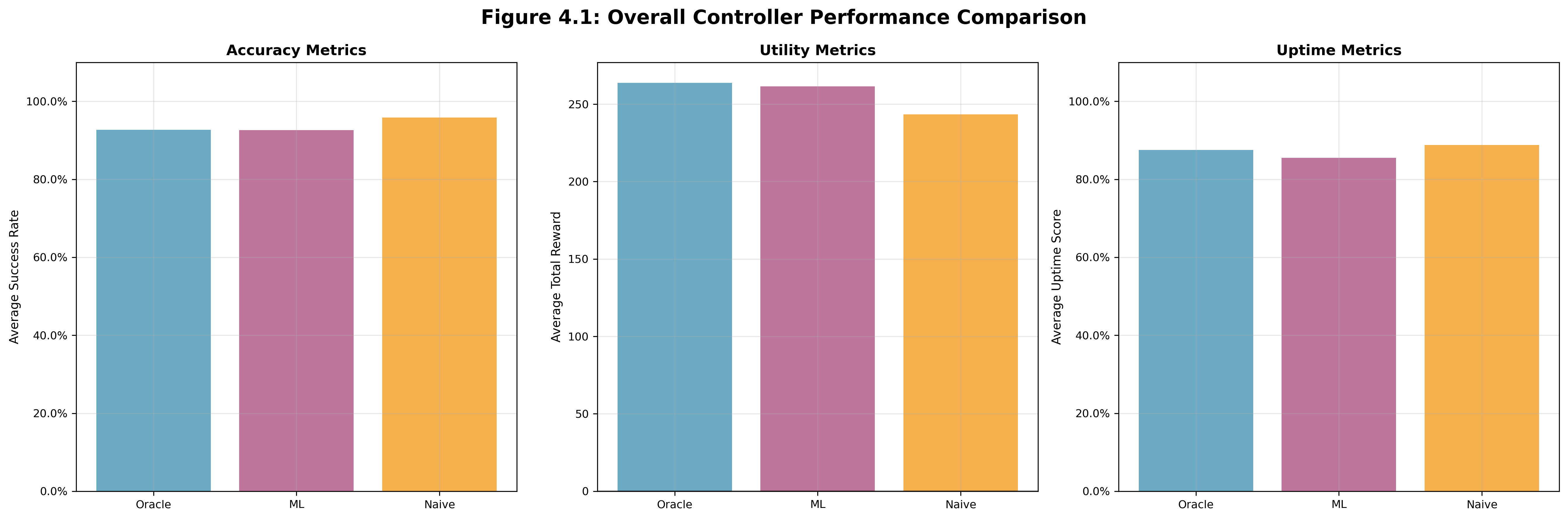
Figure 4.1: Average results across ALL controllers.
We can clearly see that the custom controller going toe-to-toe with the other 2 controllers, and even performing better than the Naive controller in terms of Utility.
4.4 Targeted Ablation Studies
Systematic ablation studies with clean parameter isolation to understand individual parameter impacts on controller performance. Each figure uses a consistent 3-panel horizontal layout showing Accuracy | Utility | Uptime metrics, as defined in Section 4.3. Unless otherwise stated, assume all information is an average of 4 simulations (1 each from 2024-2-20, 2024-5-20, 2024-8-20, 2024-11-20 respectively) of data from Southern California.
4.4.1 Accuracy & Latency
Compares controllers with different accuracy and latency thresholds to understand how user requirement stringency affects controller performance. We can see that the accuracy and latency thresholds did have a significant impact as the battery got lower and only the higher-powered models were viable. The Naive controller's aggressiveness outperformed the other two controllers handily on accuracy and uptime.
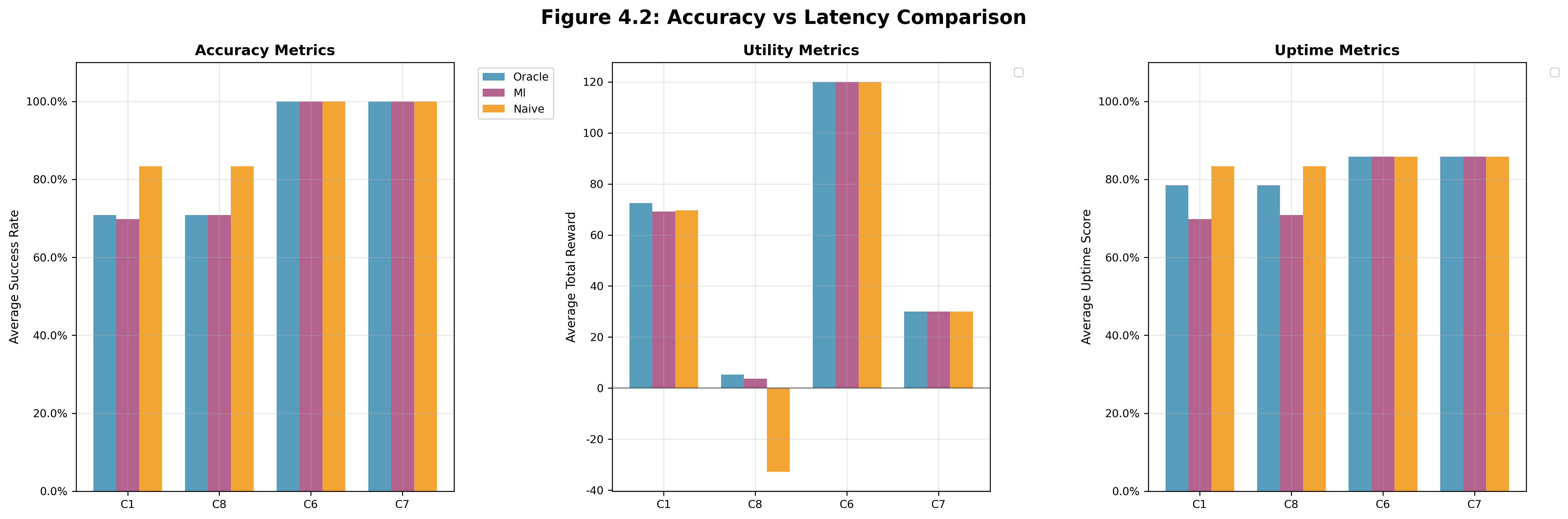
Figure 4.2 | High Accuracy & Latency (C1, C8): acc=0.95, lat=0.015s, Battery Capacity, Charging Rate = (105 mWh, 0.001598) | Low Accuracy & Latency (C6, C7): acc=0.819, lat=0.006s | Battery Capacity, Charging Rate (C1, C6, C7, C8) = (105 mWh, 0.001598)
4.4.2 Reward Weights
Compares controllers with different reward weight configurations to understand how reward design affects controller behavior. We can see that there was no inherant difference bewteen the 3 controller types due to specifically the reward metrics, as the metrics are identical per simulation parameter set.
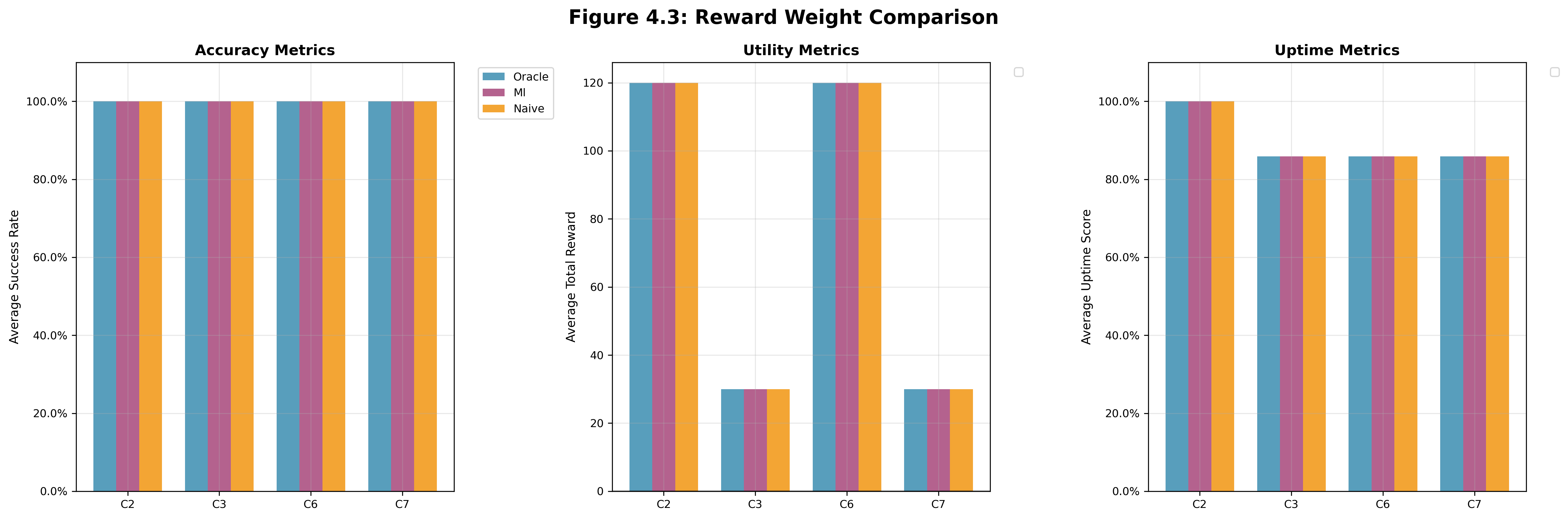
Figure 4.3 | Success-weighted (C2, C6): Performance-focused weights | Carbon-weighted (C3, C7): Carbon-focused weights | Battery Capacity, Charging Rate (C2, C3) = (610 mWh, 0.000269) | Battery Capacity, Charging Rate (C6, C7) = (105 mWh, 0.001598)
4.4.3 Battery Configuration
Compares controllers with different battery configurations to understand how hardware constraints affect controller performance. We can see that Controller 8 (Small Battery, Carbon-focused) performed more erratically than the others, suggesting that smaller batteries are not as easily adaptable to carbon-focused weights.
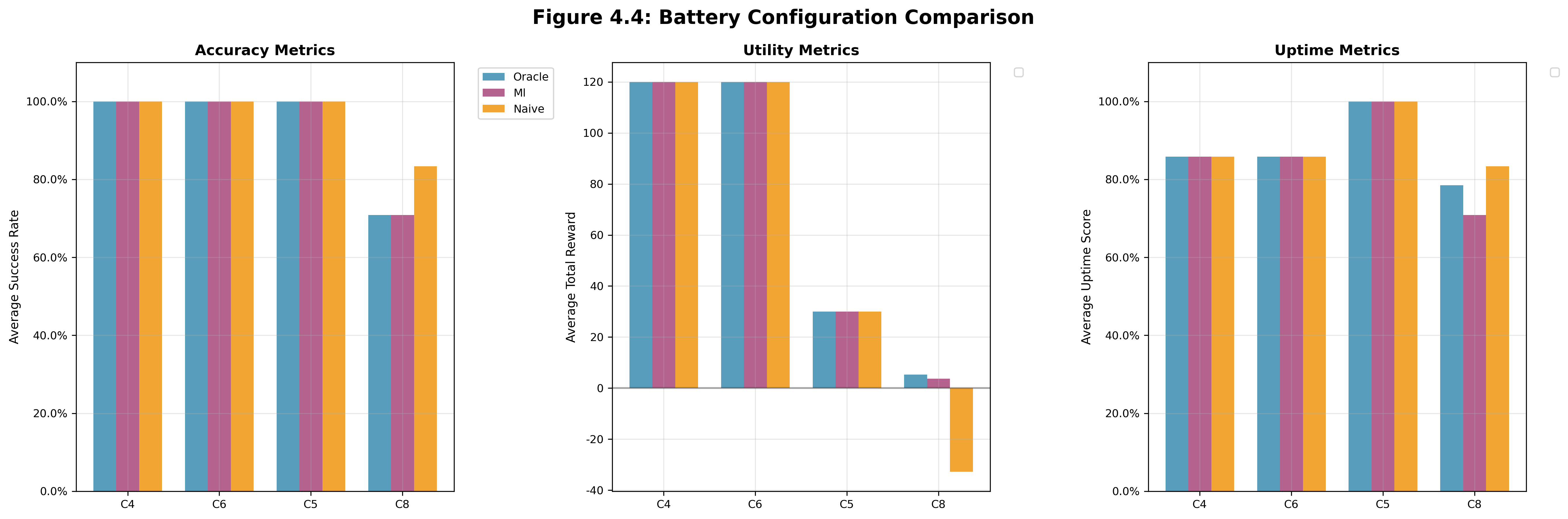
Figure 4.4 | Small Battery (C6, C8): Battery Capacity, Charging Rate = (105 mWh, 0.001598) | Large Battery (C4, C5): Battery Capacity, Charging Rate = (610 mWh, 0.000269) | Success-weighted (C4, C6): Performance-focused weights | Carbon-weighted (C5, C8): Carbon-focused weights
4.4.4 Seasonal Variation
Analyzes average controller performance across all seasonal test dates to understand how seasonal carbon intensity patterns affect overall system behavior. We can see that performance was not dependent on the season at all.
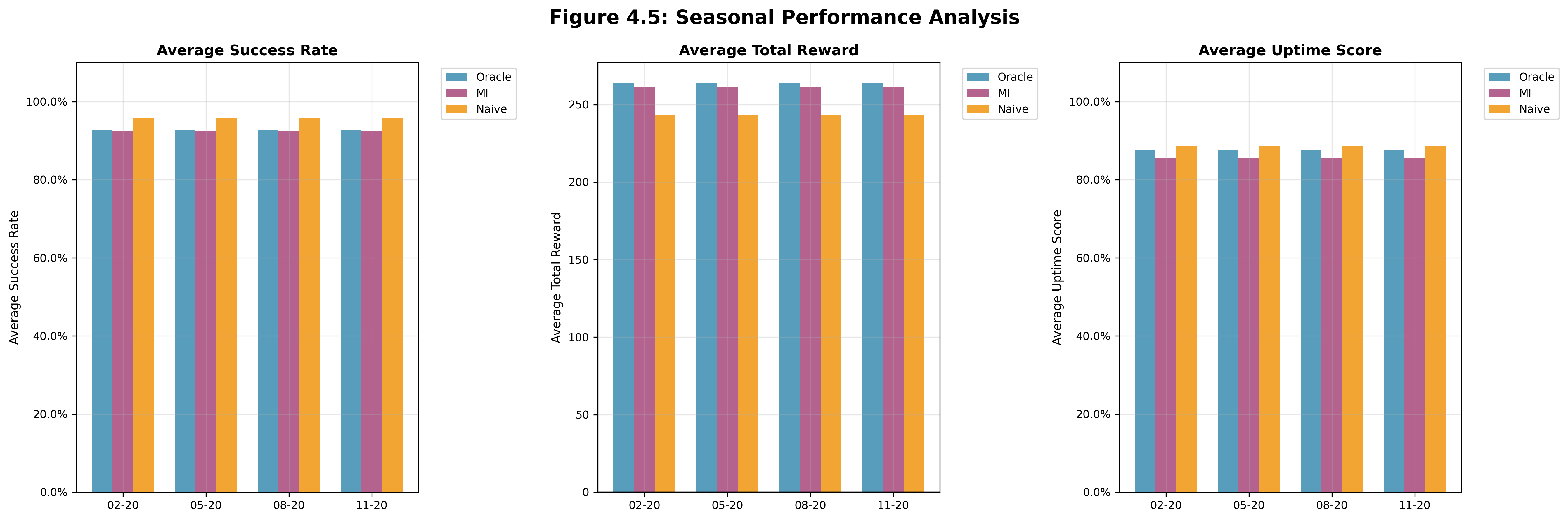
Figure 4.5 | Winter: Feb. 20th 2024 | Spring: May 20th 2024 | Summer: Aug. 20th 2024 | Autumn: Nov. 20th 2024
5. Discussion & Conclusions
5.1 What worked well and why?
The discretized oracle approach with MDP solving turned out to be a really solid baseline. Even with our coarse discretization, the oracle consistently produced feasible trajectories that respected battery constraints while optimizing the reward trade-offs, and never performed worse than the Naive controller in terms of Utility. As shown in Section 4.3 (Figure 4.1), the oracle's performance was consistently the upper bound for all experiments, as we designed it to be.
The naive controller proved to be a very strong baseline and was significantly easier to setup since it didn't require any prior data. While it did have some hiccups (see C8 data in Figure 4.2 and Figure 4.4), overall it was pretty solid when you had enough leeway in the system constraints.
Even though the training data was from California + New York, the ML controller still performed better than Naive on our California test data. This shows that the approach is carbon data independent and that other parameters like battery and user information are more important for the model's success. If we look at Figure 4.2, Figure 4.3, and Figure 4.4, we can see that the system parameters had a larger impact on the model's performance, compared to the time of year (carbon data) in Figure 4.5.
5.2 What didn't work and why?
The biggest bottleneck is the runtime cost of generating all the oracle data. Even with our discretization and K-nearest neighbor tricks, solving the MDP for multiple parameter combinations takes up so much computation time. As you can see from the training data generation parameters in Section 4.1, we were limited to just a few locations and seasonal combinations because each oracle solve took forever. This really constrained how broad our parameter coverage could be and ultimately limited how many controllers we could realistically train within the project timeline.
5.3 Limitations
Due to computational and project time constraints, our simulation engine has the following limitations:
- There is no runtime measurement of battery consumption per task; we only use the model profiles.
- Idle energy consumed by any controller is not considered. In the real world, there is some very small idle energy cost even when the controller is 'sleeping.'
- Energy and latency consumed when running the controller-selection algorithm (or running the NN to make decision) is not accounted for.
A future simulation engine would consider all the limitations above.
As mentioned numerous times above, our custom controller is specifically trained on a set of system parameters. The custom controller does not support varying the system parameters without retraining the controller. If we had more time to run the oracle on a wider range of system parameters, we would generate a massive dataset using our oracle that can train a controller to recognize the diverse requirements and parameter combinations that are possible. This would give us one general-use controller that is plug-and-play anywhere. Unfortunately, due to time constraints, we could only train a limited number of custom controllers with rigid parameters.
Due to our time constraints, we were not able to perform more ablation studies on this controller. We only had enough time to generate statistics for 1 region (Southern California). The computational cost of solving the MDP, even after the restrictions and trade-offs we made, is so large that there was not enough time to do this. This ties in to the previous point, as more abelation studies would also allow for the general controller to be trained.
5.4 Future Work
Future work could incorporate algorithms and methodology from the Data-driven Planning via Imitation Learning paper[4] to speed up our oracle training data generation. While our current approach uses basic supervised learning with cross-entropy loss, more sophisticated imitation learning techniques could improve controller performance and make the algorithms faster.
If we wanted to be simplier, we could incorperate a dual-algorithm controller, where the main policy comes from the neural-network, but the fallback policy is the same as the Naive, to get the best of both worlds.
Finally, we could also explore an always-learning LSTM-type controller that self-updates itself every task interval at runtime. This would allow a 'set-it-and-forget-it' autonomous controller that doesn't need to get retrained periodically.
6. References
Carbon- and Precedence-Aware Scheduling for Data Processing Clusters[2]
Lechowicz, A., Shenoy, R., Bashir, N., Hajiesmaili, M., Wierman, A., & Delimitrou, C. Carbon- and Precedence-Aware Scheduling for Data Processing Clusters. arXiv:2502.09717, 2025. [Paper]
Carbon-Aware Workload Management in Data Centers[3]
Nkwawir, B.W., Kayalica, M.O., Guven, D., Duman, A.C., & Erden, H.S. Carbon-Aware Workload Management in Data Centers: A Multi-Energy Integration Approach. In Proceedings of 16th ACM International Conference on Future and Sustainable Energy Systems (E-Energy '25), Association for Computing Machinery, New York, NY, USA, 907-914. [Paper]
Data-driven Planning via Imitation Learning[4]
Choudhury, S., Bhardwaj, M., Arora, S., Kapoor, A., Ranade, G., Scherer, S., & Dey, D. Data-driven Planning via Imitation Learning. The Robotics Institute, Carnegie Mellon University & Microsoft Research. [Paper]
Monte-Carlo Planning in Large POMDPs[5]
Silver, D., & Veness, J. Monte-Carlo Planning in Large POMDPs. MIT & UNSW, Sydney, Australia. [Paper]
Optimal Control of Markov Processes with Incomplete State Information I[6]
Åström, K.J. Optimal Control of Markov Processes with Incomplete State Information I. In Journal of Mathematical Analysis and Applications 10. p.174-205, 1965. [Paper]
7. Supplementary Material
7.1 Datasets
Electricity Maps grid carbon traces (external). 2024 time-series CSVs at 5-minute granularity for 4 U.S. regions from Electricity Maps, stored in energy-data/. We replay these traces in simulation as the time-varying carbon signal. Preprocessing: load CSV, sort by timestamp, select column 7 (Carbon-free energy percentage, CFE%), and align to the simulator timestep (hold the most recent 5-minute value when the task interval is finer). No labeling.
YOLOv10 model metadata (external). Per-variant accuracy and specs from Ultralytics YOLOv10 documentation used to parameterize model trade-offs in the simulator. No labeling.
Power profiling logs (internal). Our benchmark scripts generate per-model power and latency stats saved to model-profiler/power_profiles.json and used to estimate energy-per-inference.
Benchmark images (internal). Fixed images in benchmark-images/ used only to run consistent inference during profiling and simulation, not to train YOLO.
7.2 Software
External libraries: PyTorch, NumPy, Astral (uv).
External models: Ultralytics YOLOv10 variants (N/S/M/B/L/X).
Internal code: Simulation + battery model, oracle planner, training-data generation, imitation-learning controller, and profiling utilities.
AI Coding Tools: Windsurf, Claude Code, ChatGPT